Six Sigma Analyze : 1 Measuring and modeling the relationship between Variables
Simple Linear Regression Population Model Hypothesis Tests in Simple Linear Regression t-test Coefficient of Determination (R2) Confidence Intervals Multiple Linear Regression Multi-Vari Analysis Multi-Vari Sampling Plan Design Procedure Multi-Vari Case Study
Simple Linear Regression
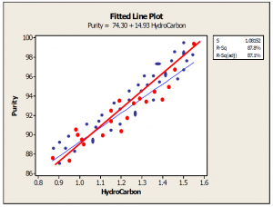
In statistics, simple linear regression is the least squares estimator of a linear regression model with a single explanatory variable. In other words, simple linear regression fits a straight line through the set of n points in such a way that makes the sum of squared residuals of the model (that is, vertical distances between the points of the data set and the fitted line) as small as possible.
The adjective simple refers to the fact that this regression is one of the simplest in statistics. The slope of the fitted line is equal to the correlation between y and x corrected by the ratio of standard deviations of these variables. The intercept of the fitted line is such that it passes through the center of mass (x, y) of the data points.
Other regression methods besides the simple ordinary least squares (OLS) also exist (see linear regression). In particular, when one wants to do regression by eye, one usually tends to draw a slightly steeper line, closer to the one produced by the total least squares method. This occurs because it is more natural for one’s mind to consider the orthogonal distances from the observations to the regression line, rather than the vertical ones as OLS method does.
Read more
Simple Linear Regression
In statistics, simple linear regression is the least squares estimator of a linear regression model with a single explanatory variable. In other words, simple linear regression fits a straight line through the set of n points in such a way that makes the sum of squared residuals of the model (that is, vertical distances between the points of the data set and the fitted line) as small as possible.
The adjective simple refers to the fact that this regression is one of the simplest in statistics. The slope of the fitted line is equal to the correlation between y and x corrected by the ratio of standard deviations of these variables. The intercept of the fitted line is such that it passes through the center of mass (x, y) of the data points.
Other regression methods besides the simple ordinary least squares (OLS) also exist (see linear regression). In particular, when one wants to do regression by eye, one usually tends to draw a slightly steeper line, closer to the one produced by the total least squares method. This occurs because it is more natural for one’s mind to consider the orthogonal distances from the observations to the regression line, rather than the vertical ones as OLS method does.
Read more
Population Model
A population model is a type of mathematical model that is applied to the study of population dynamics.
Models allow a better understanding of how complex interactions and processes work. Modeling of dynamic interactions in nature can provide a manageable way of understanding how numbers change over time or in relation to each other. Ecological population modeling is concerned with the changes in population size and age distribution within a population as a consequence of interactions of organisms with the physical environment, with individuals of their own species, and with organisms of other species. The world is full of interactions that range from simple to dynamic. Many, if not all, of Earth’s processes affect human life. The Earth’s processes are greatly stochastic and seem chaotic to the naked eye. However, a plethora of patterns can be noticed and are brought forth by using population modeling as a tool. Population models are used to determine maximum harvest for agriculturists, to understand the dynamics of biological invasions, and have numerous environmental conservation implications. Population models are also used to understand the spread of parasites, viruses, and disease. The realization of our dependence on environmental health has created a need to understand the dynamic interactions of the earth’s flora and fauna. Methods in population modeling have greatly improved our understanding of ecology and the natural world
More here
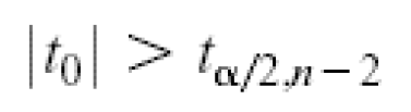
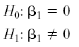
Hypothesis Tests in Simple Linear Regression
Use of t-Tests. A t-test is any statistical hypothesis test in which the test statistic follows a Student’s t-distribution if the null hypothesis is supported. It can be used to determine if two sets of data are significantly different from each other, and is most commonly applied when the test statistic would follow a normal distribution if the value of a scaling term in the test statistic were known. When the scaling term is unknown and is replaced by an estimate based on the data, the test statistic (under certain conditions) follows a Student’s t distribution.
We would reject the null hypothesis if
A population model is a type of mathematical model that is applied to the study of population dynamics.
Models allow a better understanding of how complex interactions and processes work. Modeling of dynamic interactions in nature can provide a manageable way of understanding how numbers change over time or in relation to each other. Ecological population modeling is concerned with the changes in population size and age distribution within a population as a consequence of interactions of organisms with the physical environment, with individuals of their own species, and with organisms of other species. The world is full of interactions that range from simple to dynamic. Many, if not all, of Earth’s processes affect human life. The Earth’s processes are greatly stochastic and seem chaotic to the naked eye. However, a plethora of patterns can be noticed and are brought forth by using population modeling as a tool. Population models are used to determine maximum harvest for agriculturists, to understand the dynamics of biological invasions, and have numerous environmental conservation implications. Population models are also used to understand the spread of parasites, viruses, and disease. The realization of our dependence on environmental health has created a need to understand the dynamic interactions of the earth’s flora and fauna. Methods in population modeling have greatly improved our understanding of ecology and the natural world
More here
Hypothesis Tests in Simple Linear Regression
Use of t-Tests. A t-test is any statistical hypothesis test in which the test statistic follows a Student’s t-distribution if the null hypothesis is supported. It can be used to determine if two sets of data are significantly different from each other, and is most commonly applied when the test statistic would follow a normal distribution if the value of a scaling term in the test statistic were known. When the scaling term is unknown and is replaced by an estimate based on the data, the test statistic (under certain conditions) follows a Student’s t distribution.
We would reject the null hypothesis if
|
|
These hypotheses relate to the significance of regression. Failure to reject H0 is equivalent to concluding that there is no linear relationship between xand Y.
Hypothesis testing in simple linear regression: partitioning the total sums of squares

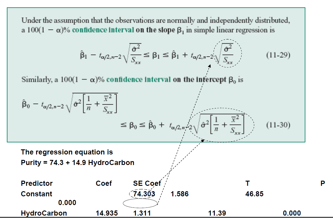
Confidence Intervals
In statistics, a confidence interval (CI) is a type of interval estimate of a population parameter. It is an observed interval (i.e., it is calculated from the observations), in principle different from sample to sample, that frequently includes the value of an un observable parameter of interest if the experiment is repeated. How frequently the observed interval contains the parameter is determined by the confidence level or confidence coefficient. More specifically, the meaning of the term “confidence level” is that, if CI are constructed across many separate data analyses of replicated (and possibly different) experiments, the proportion of such intervals that contain the true value of the parameter will match the given confidence level.Whereas two-sided confidence limits form a confidence interval, their one-sided counterparts are referred to as lower or upper confidence bounds.
Confidence intervals consist of a range of values (interval) that act as good estimates of the unknown population parameter; however, in infrequent cases, none of these values may cover the value of the parameter. It does not describe any single sample. This value is represented by a percentage, so when we say, “we are 99% confident that the true value of the parameter is in our confidence interval”, we express that 99% of the hypothetically observed confidence intervals will hold the true value of the parameter. After any particular sample is taken, the population parameter is either in the interval realized or not; it is not a matter of chance. The desired level of confidence is set by the researcher (not determined by data). If a corresponding hypothesis test is performed, the confidence level is the complement of respective level of significance, i.e. a 95% confidence interval reflects a significance level of 0.05. The confidence interval contains the parameter values that, when tested, should not be rejected with the same sample. Greater levels of variance yield larger confidence intervals, and hence less precise estimates of the parameter. Confidence intervals of difference parameters not containing 0 imply that there is a statistically significant difference between the populations.
In applied practice, confidence intervals are typically stated at the 95% confidence level. However, when presented graphically, confidence intervals can be shown at several confidence levels, for example 90%, 95% and 99%.
Certain factors may affect the confidence interval size including size of sample, level of confidence, and population variability. A larger sample size normally will lead to a better estimate of the population parameter.
The confidence interval estimate of the expected value of y will be narrower than the prediction interval for the same given value of x and confidence level. This is because there is less error in estimating a mean value as opposed to predicting an individual value.
Prediction Interval : Used to estimate the value of one value of y (at given x)
Confidence Interval : Used to estimate the mean value of y (regression line) (at given x)
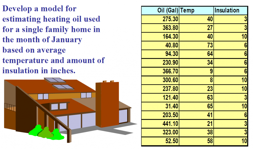
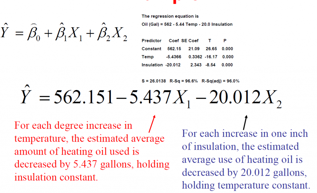
Multiple Linear Regression
In statistics, linear regression is an approach for modeling the relationship between a scalar dependent variable y and one or more explanatory variables (or independent variable) denoted X. The case of one explanatory variable is called simple linear regression. For more than one explanatory variable, the process is called multiple linear regression. (This term should be distinguished from multivariate linear regression, where multiple correlated dependent variables are predicted, rather than a single scalar variable.)
Prediction Interval : Used to estimate the value of one value of y (at given x)
Confidence Interval : Used to estimate the mean value of y (regression line) (at given x)
Multiple Linear Regression
In statistics, linear regression is an approach for modeling the relationship between a scalar dependent variable y and one or more explanatory variables (or independent variable) denoted X. The case of one explanatory variable is called simple linear regression. For more than one explanatory variable, the process is called multiple linear regression. (This term should be distinguished from multivariate linear regression, where multiple correlated dependent variables are predicted, rather than a single scalar variable.)
Multi-Vari Analysis
In statistical process control, one tracks variables like pressure, temperature or pH by taking measurements at certain intervals. The underlying assumption is that the variables will have approximately one representative value when measured. Frequently, this is not the case. Temperature in the cross-section of a furnace will vary and the thickness of a part may also vary depending on where each measurement is taken. Often the variation is within piece and the source of this variation is different from piece-to-piece and time-to-time variation. The multi-varichart is a very useful tool for analyzing all three types of variation. Multi-varicharts are used to investigate the stability or consistency of a process. The chart consists of a series of vertical lines, or other appropriate schematics, along a time scale. The length of each line or schematic shape represents the range of values found in each sample set.
Multi-Vari Sampling Plan Design Procedure
1.Select the process and the characteristic to be investigated.
2. Select the sample size and time frequency.
3. Set up a tabulation sheet to record the time and values from each sample set.
4. Plot the multi-varichart on graph paper with time along the horizontal scale and the measured values on the vertical scale.
5. Join the observed values with appropriate lines.
6. Analyze the chart for variation both within the sample set, from sample to sample and over time.
7. It may be necessary to conduct additional studies to concentrate on the area(s) of apparent maximum variation.
8. After process improvements, it will be necessary to repeat the multi-varistudy to confirm the results.
Step-by-step procedure of the MultiVariChart Analysis:
1. Identify the single unit in which a set of multivariate data is collected, and select a good data collection plan so that each data set contains sufficient information for our study.
2. Select an appropriate graphical data visualization scheme. The selected data visualization scheme should provide problem analysts sufficient information to assess the magnitude of variation and the mutual relationship among multivariate variables, and the ‘signature’of the visualization should provides powerful clues for root cause analysis.
3. Select the inclusive categories of variations, for which all types of variations can be partitioned into these categories. The category partition of intra-piece, inter-piece and time to time is one such an example.
4. Collect multivariate data samples, and display the data visualization graphs under each category.
5. Determine the major category(ies) that accommodate most of variation, and using subject of matter knowledge to unlock the root cause of variation in that category.
Multi-Vari Case Study
A manufacturer produced flat sheets of aluminum on a hot rollingmill. Although a finish trimming operation followed, the basic aluminum plate thickness was established during the rolling operation. The thickness specification was 0.245″ to.005″. The operation had been producing scrap. A process capability study indicated that the process spread was 0.0125″ (a Cp of 0.8) versus the requirement of 0.010″. The operation generated a profit of approximately $200,000 per month even after a scrap loss of $20,000 per month.
Refitting the mill with a more modern design, featuring automatic gauge control and hydraulic roll bending, would cost $800,000 and result in 6 weeks of downtime for installation. The department manager requested that a multi-vari study be conducted by a quality engineer before further consideration of the new mill design or other alternatives. Four positional measurements were made at the corners of each flat sheet in order r to adequately determine within piece variation. Three flat sheets were measured in consecutive order to determine piece to piece variation. Additionally, samples were collected each hour to determine temporal variation.
The results of this short term study were slightly better than the earlier process capability study. The maximum detected variation was 0.010″. Without sophisticated analysis, it appeared that the time to time variation was the largest culprit. A gross change was noted after the 10:00 AM break.
During this time, the roll coolant tank was refilled. Actions taken over the next two weeks included re-leveling the bottom back-up roll (approximately 30% of total variation) and initiating more frequent coolant tank additions, followed by an automatic coolant make-up modification (50% of total variation). Additional spray nozzles were added to the roll stripper housings to reduce heat build up in the work rolls during the rolling process (10-15% of total variation). The piece to piece variation was ignored. This dimensional variation may have resulted from roll bearing slop or variation in incoming aluminum sheet temperature (or a number of other sources).
The results from this single study indicated that, if all of the modifications were perfect, the resulting measurement spread would be 0.002″ total.In reality, the end result was : +/-0.002″ or 0.004″ total, under conditions similar to that of the initial study. The total cash expenditure was $8,000 for the described modifications. All work was completed in two weeks. The specification of 0.245″ +/-0.005″ was easily met. Most multi-vari analysis does not yield results that are this spectacular, but the potential for significant improvement is apparent.